Plotting the per base coverage of genomic features
The kpPlotBAMCoverage function is similar to
kpPlotCoverage
but instead of plotting the coverage of genomic regions stored in as an R
object it will plot the coverage of a BAM file. This function plots the actual
base-level coverage and so it’s use is limited to relatively small regions.
By default it will error if we try to plot a region larger than 1Mb, but
this is configurable and with sufficient time and memory there should be no
hard limit the size of the plot region, we simply should change the
max.valid.region.size to the size of the region we want to plot.
However, if we want to plot a global view of coverage along the whole genome,
for example, we should consider using
kpPlotBAMDensity
instead, which is much faster. kpPlotBAMCoverage can be used to plot the
coverage of BAM files for any experiment on any genome.
As an example, we’ll use the BAM files for an RNA-seq experiment in flies contained in the Bioconductor package pasillaBamSubset. This package contains 2 BAM files with RNA-seq data from 2 differents samples restricted to only data in chromosome chr4, the shortest one in Drosophila’s genome. The package defines two functions that return the paths to the BAM files.
library(pasillaBamSubset)

bam1 <- untreated1_chr4()
bam2 <- untreated3_chr4()
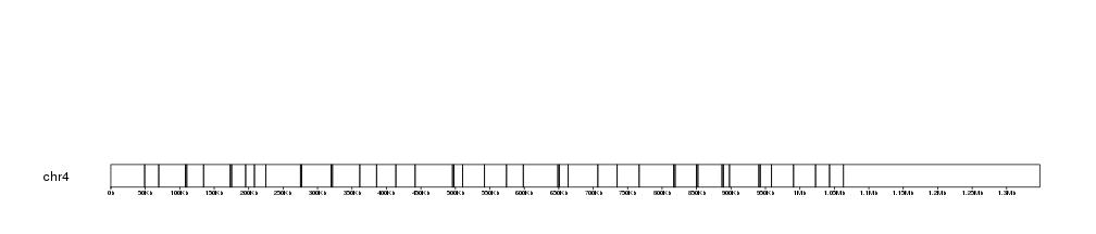
To plot them we will create a karyoplot of the chr4 of the Drosophila’s genome
version dm6.
library(karyoploteR)

kp <- plotKaryotype(genome = "dm6", chromosomes = "chr4")
kpAddBaseNumbers(kp, tick.dist = 50000, add.units = TRUE)

And plot it simply using giving the name of the file to the function
kp <- plotKaryotype(genome = "dm6", chromosomes = "chr4")
kpAddBaseNumbers(kp, tick.dist = 50000, add.units = TRUE)
kp <- kpPlotBAMCoverage(kp, data=bam1)
## Warning in kpPlotBAMCoverage(kp, data = bam1): In kpPlotBAMCoverage: Skipping BAM coverage plot.
## The genomic region in your plot is larger than the maximum
## valid size. Plotting coverage in a very large region would
## probably result in very large memory usage and potentially
## crash your R session while creating not very informative
## plots. For larger regions, kpPlotBAMDensity is recommended.
## If you want to plot the coverage in a large region,
## please supply a larger value for 'max.valid.region.size'
## parameter.
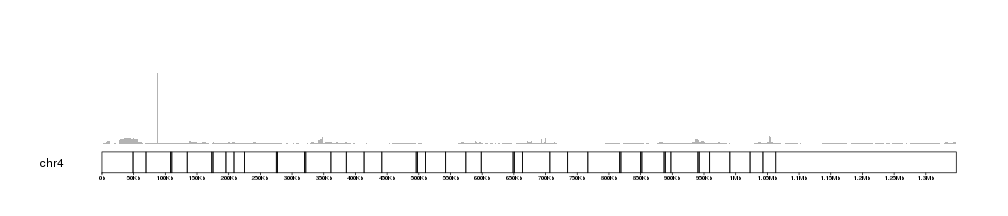
We get a warning and the BAM coverage is not plotted. This is because the chr4 is larger than the maximum default size allowed. To plot we can increase it, for example to 2Mb, and we should get our plot.
kp <- plotKaryotype(genome = "dm6", chromosomes = "chr4")
kpAddBaseNumbers(kp, tick.dist = 50000, add.units = TRUE)
kp <- kpPlotBAMCoverage(kp, data=bam1, max.valid.region.size = 2e6)
If no ymax is given, the plot will adjust itself to the height of the highest
coverage peak. We can retrieve this value using the latest.plot info
stored in kp by some plotting functions.
kp$latest.plot$computed.values$max.coverage
## [1] 5627
And this value might be very useful to create automatic axis to our BAM coverage plots.
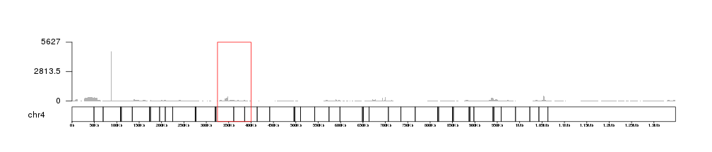
kp <- plotKaryotype(genome = "dm6", chromosomes = "chr4")
kpAddBaseNumbers(kp, tick.dist = 50000, add.units = TRUE)
kp <- kpPlotBAMCoverage(kp, data=bam1, max.valid.region.size = 2e6)
kpAxis(kp, ymax=kp$latest.plot$computed.values$max.coverage)
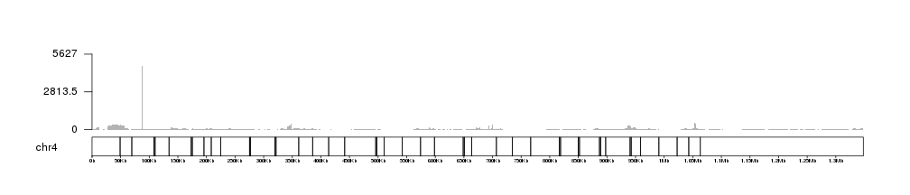
We can see that there is a single veeeery high peak that dominates the plot.
If we zoom in into other parts of the chromosome the ymax value will
autoadjust. For example, we can concentrate on the region between 325Kb and
400Kb.
kp <- plotKaryotype(genome = "dm6", chromosomes = "chr4")
kpAddBaseNumbers(kp, tick.dist = 50000, add.units = TRUE)
kp <- kpPlotBAMCoverage(kp, data=bam1, max.valid.region.size = 2e6)
kpAxis(kp, ymax=kp$latest.plot$computed.values$max.coverage)
kpRect(kp, chr="chr4", x0=325000, x1=400000, y0=0, y1=1, border="red", col=NA, data.panel = "all")
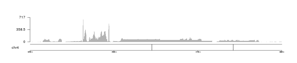
and zoom in using zoom, we can see how the coverage and the axis adjust themselves to the new maximum coverage in the region.
kp <- plotKaryotype(genome = "dm6", chromosomes = "chr4", zoom=toGRanges("chr4:325000-400000"))
kpAddBaseNumbers(kp, tick.dist = 25000, add.units = TRUE)
kp <- kpPlotBAMCoverage(kp, data=bam1)
kpAxis(kp, ymax=kp$latest.plot$computed.values$max.coverage)
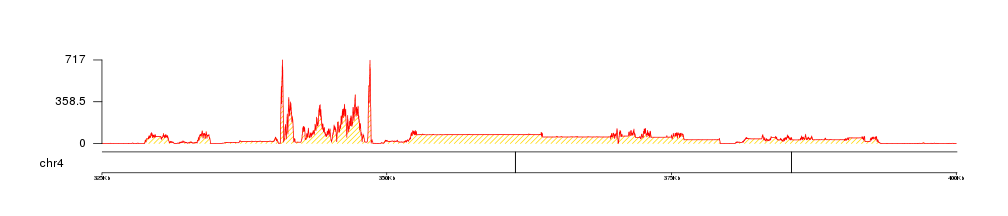
We can apply the standard customization options such as colors using the same parameters we use for other potting functions. In particular, kpPlotBAMCoverage uses kpArea behind the scenes, so it can be customized using the any parameter accepted by it.
kp <- plotKaryotype(genome = "dm6", chromosomes = "chr4", zoom=toGRanges("chr4:325000-400000"))
kpAddBaseNumbers(kp, tick.dist = 25000, add.units = TRUE)
kp <- kpPlotBAMCoverage(kp, data=bam1, col="gold", border="red", density=20)
kpAxis(kp, ymax=kp$latest.plot$computed.values$max.coverage)
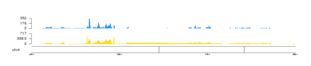
In addition, we can use r0 and r1 to control the vertical positioning of the data, so we can plot multiple file in a single plot.
IMPORTANT: If you are modifying the data positioning parameters in any way, the kpAxis statements should be changed accordingly!
kp <- plotKaryotype(genome = "dm6", chromosomes = "chr4", zoom=toGRanges("chr4:325000-400000"))
kpAddBaseNumbers(kp, tick.dist = 25000, add.units = TRUE)
kp <- kpPlotBAMCoverage(kp, data=bam1, col="#FFD700", border=NA, r1=0.4)
kpAxis(kp, ymax=kp$latest.plot$computed.values$max.coverage, r1=0.4)
kp <- kpPlotBAMCoverage(kp, data=bam2, col="#1E90FF", border=NA, r0=0.6)
kpAxis(kp, ymax=kp$latest.plot$computed.values$max.coverage, r0=0.6)
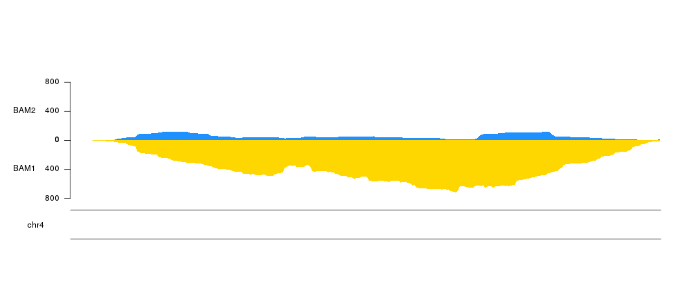
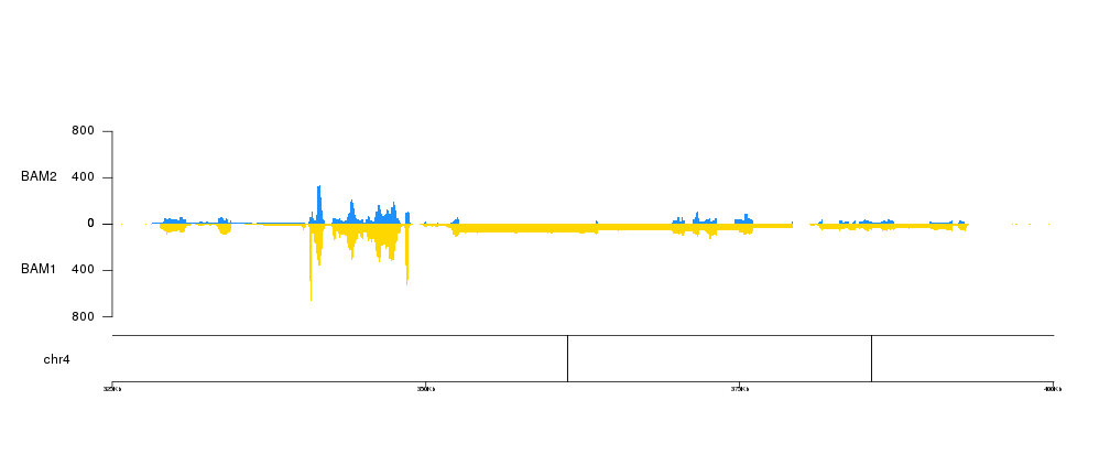
Or even us them to invert one of the plots
kp <- plotKaryotype(genome = "dm6", chromosomes = "chr4", zoom=toGRanges("chr4:325000-400000"))
kpAddBaseNumbers(kp, tick.dist = 25000, add.units = TRUE)
kp <- kpPlotBAMCoverage(kp, data=bam1, col="#FFD700", border=NA, r0=0.5, r1=0, ymax=800)
kpAxis(kp, r0=0.5, r1=0, ymax=800)
kpAddLabels(kp, "BAM1", r0=0, r1=0.5, label.margin = 0.05)
kp <- kpPlotBAMCoverage(kp, data=bam2, col="#1E90FF", border=NA, r0=0.5, r1=1, ymax=800)
kpAxis(kp, r0=0.5, r1=1, ymax=800)
kpAddLabels(kp, "BAM2", r0=0.5, r1=1, label.margin = 0.05)
Since the data plotted is the actual per-base coverage we can zoom in into a very small region and still see the actual coverage. For example showing only 300 base pairs we can see the actual coverage of each sample
kp <- plotKaryotype(genome = "dm6", chromosomes = "chr4", zoom=toGRanges("chr4:340650-340950"))
kpAddBaseNumbers(kp, tick.dist = 25000, add.units = TRUE)
kp <- kpPlotBAMCoverage(kp, data=bam1, col="#FFD700", border=NA, r0=0.5, r1=0, ymax=800)
kpAxis(kp, r0=0.5, r1=0, ymax=800)
kpAddLabels(kp, "BAM1", r0=0, r1=0.5, label.margin = 0.05)
kp <- kpPlotBAMCoverage(kp, data=bam2, col="#1E90FF", border=NA, r0=0.5, r1=1, ymax=800)
kpAxis(kp, r0=0.5, r1=1, ymax=800)
kpAddLabels(kp, "BAM2", r0=0.5, r1=1, label.margin = 0.05)