Data Positioning in karyoploteR
In karyoploteR, data is plotted in data panels. By default, the y axis of a data panels spans from 0 to 1, although this can be changed when creating the karyoplot with plot.params.
library(karyoploteR)

kp <- plotKaryotype(chromosomes="chr1")
kpDataBackground(kp)
kpAxis(kp)
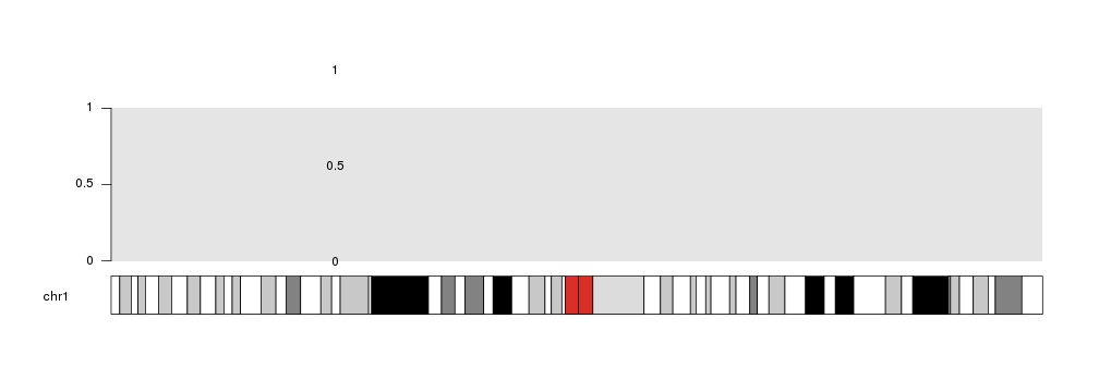
Therefore, if no additional parameters are specified when plotting data on a panel, 0 will be the bottom (actually, the closest to the ideogram), 1 the furthest and 0.5 the midpoint.
mydata <- toGRanges(data.frame(chr=rep("chr1", 3), start=rep(60e6, 3), end=rep(60e6, 3), y=c(0, 0.5, 1)))

kp <- plotKaryotype(chromosomes="chr1")
kpDataBackground(kp)
kpAxis(kp)

kpText(kp, data=mydata,  labels=c(0, 0.5, 1))
ymin and ymax
With ymin and ymax we can set a different minimum and maximum value for the current plotting call. Using these parameters WILL NOT change the default values of the data panel. That adds flexibility to the process and allows to accomodate for different scenarios, but it can create inconsitencies in the data representation if used without care. For those with experience with Circos, these parameters are equivalent to min and max in it.
For example, if we specify ymax=2, the midpoint will then be 1.
kp <- plotKaryotype(chromosomes="chr1")
kpDataBackground(kp)
kpAxis(kp)

kpText(kp, data=mydata,  labels=c(0, 0.5, 1), ymax=2)
Take into account that plotting is NOT restricted to the data panels, and might happen out of them depending on the data and the data positioning parameters.
For example, if we set ymax to 0.8, the point at 1 will fall out of the data panel. This might be useful in some situation, but it is generally not recommended.
kp <- plotKaryotype(chromosomes="chr1")
kpDataBackground(kp)
kpAxis(kp)

kpText(kp, data=mydata,  labels=c(0, 0.5, 1), ymax=0.8)
r0 and r1
r0 and r1 are two key parameters for data positioning. They are inspired in the Circos parameters with the same name specifying the radius where a plot takes place. In this case, they specify the vertical part of the data panel where the plotting should take place. They can be used to plot different data in different positions as if there were tracks.
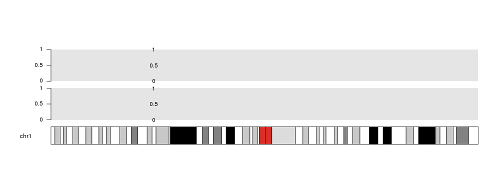
For example, we can plot 2 backgrounds in different vertical regions: one from 0 to 0.45 and one from 0.55 to 1 and plot the points in both of them.
kp <- plotKaryotype(chromosomes="chr1")
kpDataBackground(kp, r0=0, r1=0.45)
kpAxis(kp, r0=0, r1=0.45)
kpText(kp, data=mydata,  labels=c(0, 0.5, 1), r0=0, r1=0.45)

kpDataBackground(kp, r0=0.55, r1=1)
kpAxis(kp, r0=0.55, r1=1)
kpText(kp, data=mydata,  labels=c(0, 0.5, 1), r0=0.55, r1=1)
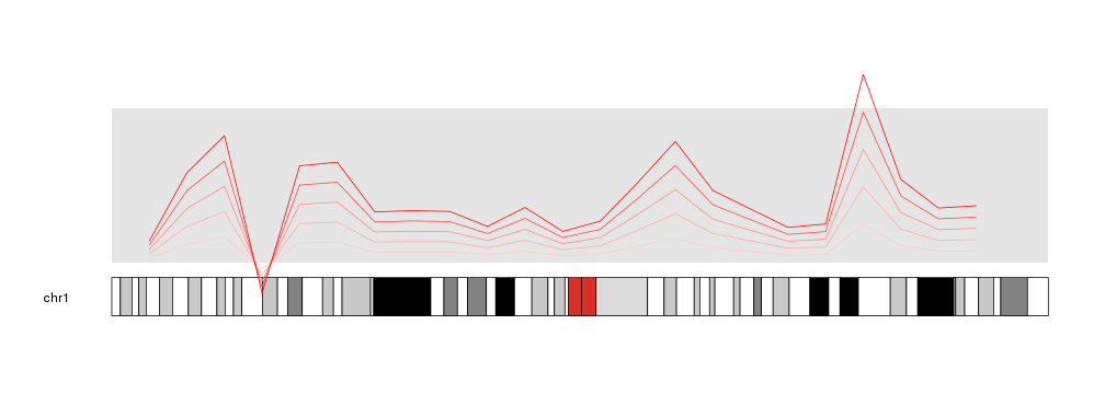
All plotting functions in karyoploteR accept these parameters and they make the plotting process very flexible.
x <- c(1:23*10e6)
y <- rnorm(n = 23, mean = 0.5, sd=0.3)

kp <- plotKaryotype(chromosomes="chr1")
kpDataBackground(kp)

kpLines(kp, chr="chr1", x=x, y=y, r1=0.2, col="#FFCCCC")
kpLines(kp, chr="chr1", x=x, y=y, r1=0.4, col="#FFAAAA")
kpLines(kp, chr="chr1", x=x, y=y, r1=0.6, col="#FF8888")
kpLines(kp, chr="chr1", x=x, y=y, r1=0.8, col="#FF4444")
kpLines(kp, chr="chr1", x=x, y=y, r1=1, col="#FF0000")
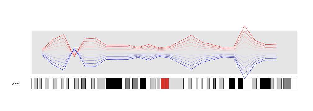
Inverting plots
An interesting usage of these parameters is to invert (flip upside down) a plot. With it is possible to create effects that would need to modify the data otherwise. To achieve that, one simply needs to specify an r0 higher than r1.
kp <- plotKaryotype(chromosomes="chr1")
kpDataBackground(kp)

kpLines(kp, chr="chr1", x=x, y=y, r0=0.5, r1=0.6, col="#FFCCCC")
kpLines(kp, chr="chr1", x=x, y=y, r0=0.5, r1=0.7, col="#FFAAAA")
kpLines(kp, chr="chr1", x=x, y=y, r0=0.5, r1=0.8, col="#FF8888")
kpLines(kp, chr="chr1", x=x, y=y, r0=0.5, r1=0.9, col="#FF4444")
kpLines(kp, chr="chr1", x=x, y=y, r0=0.5, r1=1, col="#FF0000")

kpLines(kp, chr="chr1", x=x, y=y, r0=0.5, r1=0.4, col="#CCCCFF")
kpLines(kp, chr="chr1", x=x, y=y, r0=0.5, r1=0.3, col="#AAAAFF")
kpLines(kp, chr="chr1", x=x, y=y, r0=0.5, r1=0.2, col="#8888FF")
kpLines(kp, chr="chr1", x=x, y=y, r0=0.5, r1=0.1, col="#4444FF")
kpLines(kp, chr="chr1", x=x, y=y, r0=0.5, r1=0, col="#0000FF")