Low-level plotting functions
Plotting functions in karyoploteR are divided in two groups: low- and high-level. Low level plotting functions are mainly chromosome-aware versions of the R base graphics primitives: points, lines, segments, polygons… and they do not compute anything and know nothing about biology or complex bioconductor objects.
They all share the same naming scheme: kpPrimitive, that means, kpPoints to plot points, kpLines to plot lines, kpArrows for arrows, etc. All of them are customizable using the standrad R base graphical parameters and all of them share almost the same API.
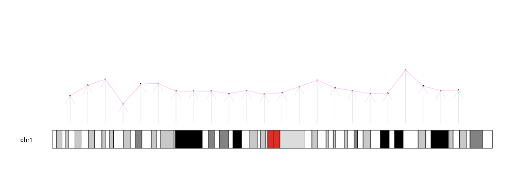
To use them, we first need to create a karyoplot with a call to plotKaryotype. After that, successive calls to the plotting functions will add new graphical elements to the plot.
library(karyoploteR)

x <- 1:23*10e6
y <- rnorm(23, 0.5, 0.1)

kp <- plotKaryotype(chromosomes="chr1")

kpPoints(kp, chr = "chr1", x=x, y=y)
kpText(kp, chr="chr1", x=x, y=y, labels=c(1:23), pos=3)
kpLines(kp, chr="chr1", x=x, y=y, col="#FFAADD")

kpArrows(kp, chr="chr1", x0=x, x1=x, y0=0, y1=y, col="#DDDDDD")
Common parameters
The low-level plotting functions can, again, be classified in two groups: those that need a single point specified by x and y (such as points, lines, text…) and those that need pair of points (x0, x1, y0, y1): segments, arrows, bars, polygons, etc. Some of the functions have special parameters, such as labels in kpText. In addition, all functions need a chr parameter to fully specify the position of each data point and the karyoplot object returned by plotKaryotype as the first parameter.
In addition to that, all functions accept a standard set of parameters to further modify the data positioning. These parameters are explained in the next section.
The data parameter
There is a special convenience parameter called data. With it, it’s possible to use a GRanges object to provide in a single object the needed data to the plotting functions. x, x0 and x1 will be derived from the start and end of the ranges in data, y, y0 and y1 from the mcols annotation, as well labels and other specific parameters. If any of this parameters is explicitly passed, it will be used instead of the one from data.
For example, we can create a GRanges object with the data used in the previous plot
mydata <- toGRanges(data.frame(chr=rep("chr1", 23), start=x, end=x, y=y))
head(mydata)
## GRanges object with 6 ranges and 1 metadata column:
##       seqnames    ranges strand |                 y
##          <Rle> <IRanges>  <Rle> |         <numeric>
##   [1]     chr1  10000000      * | 0.379293425061458
##   [2]     chr1  20000000      * | 0.527742924211066
##   [3]     chr1  30000000      * | 0.608444117668306
##   [4]     chr1  40000000      * | 0.265430229737065
##   [5]     chr1  50000000      * | 0.542912468881105
##   [6]     chr1  60000000      * | 0.550605589215757
##   -------
##   seqinfo: 1 sequence from an unspecified genome; no seqlengths
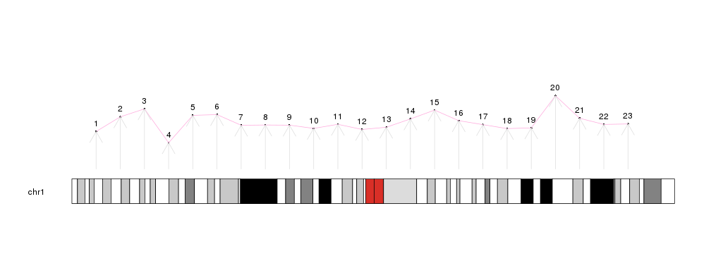
And create the same plot using this object, except for the arrows where we have to specify the y0 and y1 values since the columns in data need to have the same names as the parameters they stand for.
kp <- plotKaryotype(chromosomes="chr1")

kpPoints(kp, data=mydata)
kpText(kp, data=mydata, pos=3)
kpLines(kp, data=mydata, col="#FFAADD")

kpArrows(kp, data=mydata, y0=0, y1=y, col="#DDDDDD")
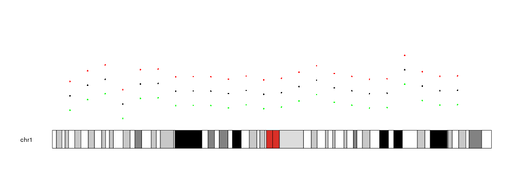
And in all cases, if y, y0 or y1 are explicitly stated, they will take precedence before the values derived from data
kp <- plotKaryotype(chromosomes="chr1")

kpPoints(kp, data=mydata)
kpPoints(kp, data=mydata, y=y+0.2, col="red")
kpPoints(kp, data=mydata, y=y-0.2, col="green")