Plotting Genomic Regions
The function kpPlotRegions as its name suggest, can be used to plot regions
along the genome. Regions are plotted as rectangles and the function includes
an option (active by default) to plot overlapping regions as a stack. This
function only accepts regions as GRanges objects and does not accept
the chr, x0, x1, y0 and y2 parameters used by kpRect.
We will create a set of random regions using
regioneR’s
createRandomRegions function and plot them on the genome.
library(karyoploteR)
regions <- createRandomRegions(nregions=400, length.mean = 3e6, mask=NA, non.overlapping = FALSE)
kp <- plotKaryotype()
kpPlotRegions(kp, data=regions)
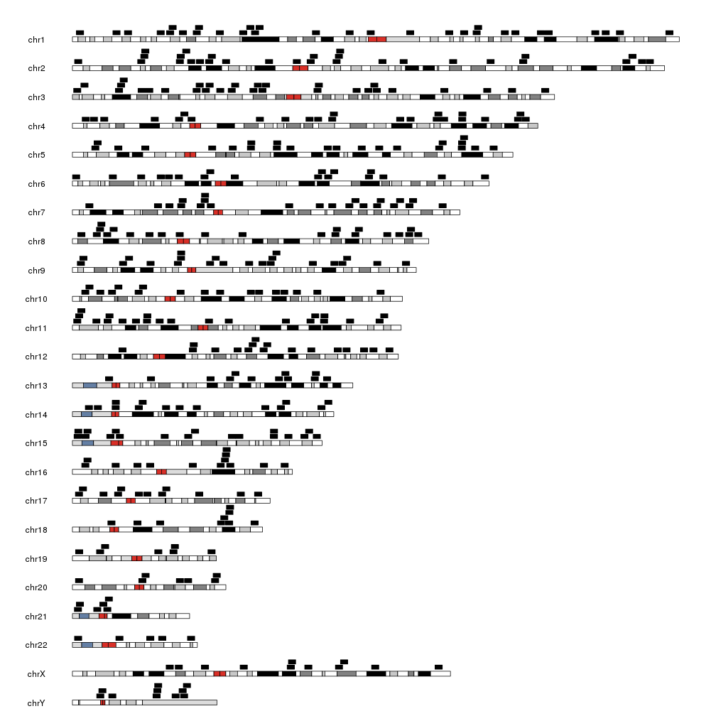
The height of the rectangles is adjusted so the tallest pile of regions fits in the data panel, making the regions flatter if needed. For example, plotting 40K regions produces a plot like this.
many.regions <- createRandomRegions(nregions=40000, length.mean = 3e6, mask=NA, non.overlapping = FALSE)
kp <- plotKaryotype()
kpPlotRegions(kp, data=many.regions)

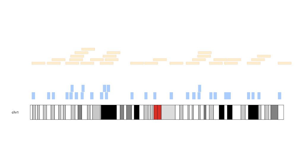
It is possible to customize the appearance of the regions using the same parameters used for kpRect plus the additional parameters avoid.overlapping, num.layers and layer.margin to control the layering of the regions.
kp <- plotKaryotype(chromosomes="chr1")
kpPlotRegions(kp, data=regions, col="#AACCFF", layer.margin = 0.01, border=NA, r0=0, r1=0.5)
kpPlotRegions(kp, data=extendRegions(regions, extend.end = 10e6), col="#FFEECC", layer.margin = 0.05, border="#FFCCAA", r0=0.6, r1=1)
Input Regions
As in most functions in karyoploteR, kpPlotRegions uses internally the
toGRangesfunction from
regioneR. This means that it’s
possible to call kpPlotRegions with a bed-like file, even a remote one,
a data.frame or even an array of characters defining the regions. You can find
more information on the valid formats in
regioneR’s vignette.
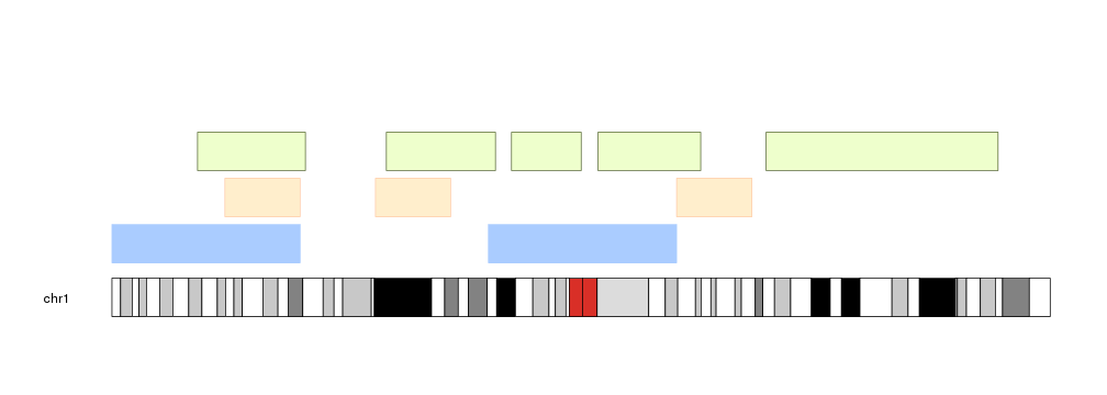
kp <- plotKaryotype(chromosomes="chr1")
kpPlotRegions(kp, data=c("chr1:1-50000000", "chr1:100e6-150e6"), col="#AACCFF", r0=0, r1=0.25)
df <- data.frame(chr=c("chr1", "chr1", "chr1"), start=c(30e6, 70e6, 150e6), end=c(50e6, 90e6, 170e6))
kpPlotRegions(kp, data=df, col="#FFEECC", border="#FFCCAA", r0=0.3, r1=0.55)
kpPlotRegions(kp, data="Tutorial/PlotRegions/regions.txt", col="#EEFFCC", border=darker("#EEFFCC"), r0=0.6, r1=0.85)