Automated Data Positioning in karyoploteR
As seen in the
data positioning
section, r0and r1can be used to define the vertical regions of the
data panels where a function will plot.
While in many cases we will manually define the r0 and r1 values, in some
circumstances it can be useful to have an automatic way of computing them.
This is the mission of the autotrack function.
autotrack will help us partition the vertical space in a number of equally
sized “tracks”, separated by a small margin.
Each call to autotrack will give us the r0 and r1 values for one of these
tracks.
For example, if we want to partition the data panel into 4 tracks and get the
r0and r1 for the first (the bottom) one, we will use this:
library(karyoploteR)

autotrack(current.track = 1, total.tracks = 4)
## $r0
## [1] 0
##
## $r1
## [1] 0.2375
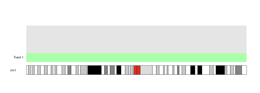
We can then use this object to set the r0and r1 in any plotting function:
kp <- plotKaryotype(chromosomes = "chr1")
kpDataBackground(kp)
at <- autotrack(current.track = 1, total.tracks = 4)
kpDataBackground(kp, r0=at$r0, r1=at$r1, color = "#AAFFAA")
kpAddLabels(kp, labels = "Track 1", r0=at$r0, r1=at$r1)
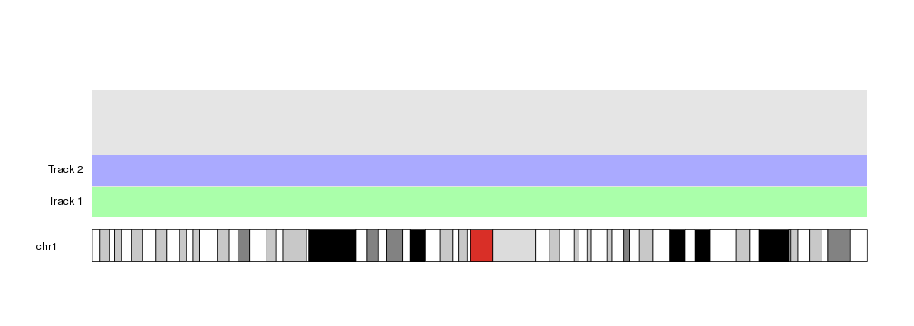
Changing the value of current.track we can then get the vertical position of
the second track.
kp <- plotKaryotype(chromosomes = "chr1")
kpDataBackground(kp)
at <- autotrack(current.track = 1, total.tracks = 4)
kpDataBackground(kp, r0=at$r0, r1=at$r1, color = "#AAFFAA")
kpAddLabels(kp, labels = "Track 1", r0=at$r0, r1=at$r1)

at <- autotrack(current.track = 2, total.tracks = 4)
kpDataBackground(kp, r0=at$r0, r1=at$r1, color = "#AAAAFF")
kpAddLabels(kp, labels = "Track 2", r0=at$r0, r1=at$r1)
The current.margin parameter can be not a single integer but an array
of integers. In that case, it will return the r0 at the bottom of the
track corresponding to the minimum of the values, and r1 corresponding to
the top of the maximum one.
kp <- plotKaryotype(chromosomes = "chr1")
kpDataBackground(kp)
at <- autotrack(current.track = 1, total.tracks = 4)
kpDataBackground(kp, r0=at$r0, r1=at$r1, color = "#AAFFAA")
kpAddLabels(kp, labels = "Track 1", r0=at$r0, r1=at$r1)
at <- autotrack(current.track = 2, total.tracks = 4)
kpDataBackground(kp, r0=at$r0, r1=at$r1, color = "#AAAAFF")
kpAddLabels(kp, labels = "Track 2", r0=at$r0, r1=at$r1)
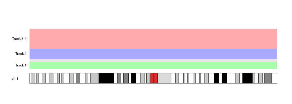
at <- autotrack(current.track = c(3,4), total.tracks = 4)
kpDataBackground(kp, r0=at$r0, r1=at$r1, color = "#FFAAAA")
kpAddLabels(kp, labels = "Track 3-4", r0=at$r0, r1=at$r1)
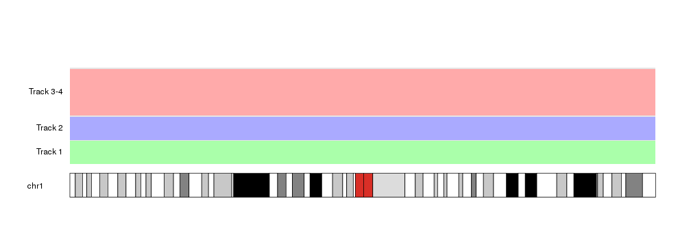
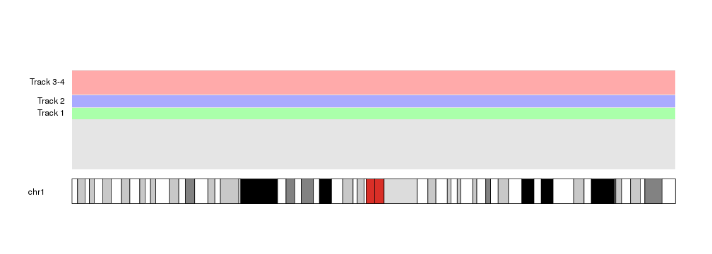
As you can see, there’s a small margin between tracks. By default it is 0.05, that is, a 5% of the total space for each track. We can modify it or remove it completely setting it to 0.
kp <- plotKaryotype(chromosomes = "chr1")
kpDataBackground(kp)
at <- autotrack(current.track = 1, total.tracks = 4, margin = 0.3)
kpDataBackground(kp, r0=at$r0, r1=at$r1, color = "#AAFFAA")
kpAddLabels(kp, labels = "Track 1", r0=at$r0, r1=at$r1)

at <- autotrack(current.track = 2, total.tracks = 4, margin = 0)
kpDataBackground(kp, r0=at$r0, r1=at$r1, color = "#AAAAFF")
kpAddLabels(kp, labels = "Track 2", r0=at$r0, r1=at$r1)

at <- autotrack(current.track = c(3,4), total.tracks = 4)
kpDataBackground(kp, r0=at$r0, r1=at$r1, color = "#FFAAAA")
kpAddLabels(kp, labels = "Track 3-4", r0=at$r0, r1=at$r1)
In addition to that, autotrack accepts its own r0and r1 parameters,
indicating the total vertical space to use for the tracks.
For example, we can repeat the example above but using only the top half of the data panel.
kp <- plotKaryotype(chromosomes = "chr1")
kpDataBackground(kp)
at <- autotrack(current.track = 1, total.tracks = 4, r0=0.5, r1=1)
kpDataBackground(kp, r0=at$r0, r1=at$r1, color = "#AAFFAA")
kpAddLabels(kp, labels = "Track 1", r0=at$r0, r1=at$r1)

at <- autotrack(current.track = 2, total.tracks = 4, r0=0.5, r1=1)
kpDataBackground(kp, r0=at$r0, r1=at$r1, color = "#AAAAFF")
kpAddLabels(kp, labels = "Track 2", r0=at$r0, r1=at$r1)

at <- autotrack(current.track = c(3,4), total.tracks = 4, r0=0.5, r1=1)
kpDataBackground(kp, r0=at$r0, r1=at$r1, color = "#FFAAAA")
kpAddLabels(kp, labels = "Track 3-4", r0=at$r0, r1=at$r1)
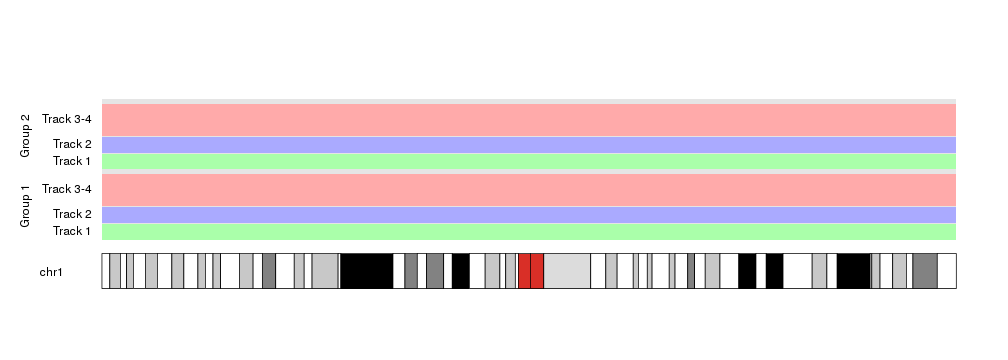
This opens the door to nested autotracks such as this
kp <- plotKaryotype(chromosomes = "chr1")
kpDataBackground(kp)

out.at <- autotrack(current.track = 1, total.tracks = 2)
kpAddLabels(kp, labels = "Group 1", pos=1, label.margin = 0.08, srt=90, r0=out.at$r0, r1=out.at$r1)
at <- autotrack(current.track = 1, total.tracks = 4, r0=out.at$r0, r1=out.at$r1)
kpDataBackground(kp, r0=at$r0, r1=at$r1, color = "#AAFFAA")
kpAddLabels(kp, labels = "Track 1", r0=at$r0, r1=at$r1)

at <- autotrack(current.track = 2, total.tracks = 4, r0=out.at$r0, r1=out.at$r1)
kpDataBackground(kp, r0=at$r0, r1=at$r1, color = "#AAAAFF")
kpAddLabels(kp, labels = "Track 2", r0=at$r0, r1=at$r1)

at <- autotrack(current.track = c(3,4), total.tracks = 4, r0=out.at$r0, r1=out.at$r1)
kpDataBackground(kp, r0=at$r0, r1=at$r1, color = "#FFAAAA")
kpAddLabels(kp, labels = "Track 3-4", r0=at$r0, r1=at$r1)


out.at <- autotrack(current.track = 2, total.tracks = 2)
kpAddLabels(kp, labels = "Group 2", pos=1, label.margin = 0.08, srt=90, r0=out.at$r0, r1=out.at$r1)
at <- autotrack(current.track = 1, total.tracks = 4, r0=out.at$r0, r1=out.at$r1)
kpDataBackground(kp, r0=at$r0, r1=at$r1, color = "#AAFFAA")
kpAddLabels(kp, labels = "Track 1", r0=at$r0, r1=at$r1)

at <- autotrack(current.track = 2, total.tracks = 4, r0=out.at$r0, r1=out.at$r1)
kpDataBackground(kp, r0=at$r0, r1=at$r1, color = "#AAAAFF")
kpAddLabels(kp, labels = "Track 2", r0=at$r0, r1=at$r1)

at <- autotrack(current.track = c(3,4), total.tracks = 4, r0=out.at$r0, r1=out.at$r1)
kpDataBackground(kp, r0=at$r0, r1=at$r1, color = "#FFAAAA")
kpAddLabels(kp, labels = "Track 3-4", r0=at$r0, r1=at$r1)
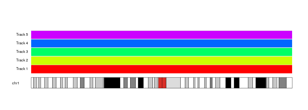
autotrack lends itself very well to be use in for loops and similar
constructs.
kp <- plotKaryotype(chromosomes = "chr1")
kpDataBackground(kp)

total.tracks <- 5
for(i in seq_len(total.tracks)) {
  at <- autotrack(current.track = i, total.tracks = total.tracks)
  kpDataBackground(kp, r0=at$r0, r1=at$r1, color = rainbow(total.tracks)[i])
  kpAddLabels(kp, labels = paste0("Track ", i), r0=at$r0, r1=at$r1)
}
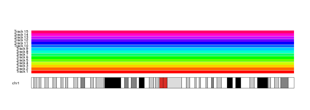
And allows for automation and parametrization
kp <- plotKaryotype(chromosomes = "chr1")
kpDataBackground(kp)

total.tracks <- 15
for(i in seq_len(total.tracks)) {
  at <- autotrack(current.track = i, total.tracks = total.tracks)
  kpDataBackground(kp, r0=at$r0, r1=at$r1, color = rainbow(total.tracks)[i])
  kpAddLabels(kp, labels = paste0("Track ", i), r0=at$r0, r1=at$r1)
}